5 September 2018 / machine learning

Sample size and class balance on model performance

tl;dr: This post shows the relationship between the sample size and the accuracy in a classification model.

I hope this little research I did may help you in your classification problems. An LSTM model created in Keras was used to produce the results.

The metric we are tracking is categorical_accuracy (equivalent to accuracy for multi-class), which is biased towards the values that have more representativeness.

For example, if we are predicting fraud, which occurs only 1 time in 1000 (0.1%); then assigning all 100% of the cases as "Non-fraud" will lead us to be correct 99.9% of the times. High, but utterly useless.

Introducing our case

I decided to study the output of this model, as a sanity check on the performance.

Each row represents a class to predict, (42 unique in total).

This is an important point, since the total different classes to predict are around 900, and the model only predicts 42. This should be a warning of the input data and/or architecture we are using, (either in Deep Learning or the "classic" Machine Learning).

Columns:

TP: True positive (the model correctly predicted the class)
rank: Indicates the rank of frequency apparition. Just like in a running competence, the fastest runner ends at the 1st place; this rank measures the order according to the class representativeness.

Loading the libraries:

# install.packages("corrr")
# install.packages("funModeling")
# install.packages("tidyverse")

library(corrr) 
library(funModeling)
library(tidyverse)

The data we are going to use looks like:

d_tp_rank=readr::read_delim("https://s3.amazonaws.com/datascienceheroes.com/img/tp_rank.csv", delim = ";")

## Parsed with column specification:
## cols(
##   TP = col_double(),
##   rank = col_integer()
## )

d_tp_rank

## # A tibble: 42 x 2
##       TP  rank
##    <dbl> <int>
##  1 0.359     1
##  2 0.312     2
##  3 0.361     3
##  4 0.14      4
##  5 0.261     5
##  6 0.216     6
##  7 0.277     7
##  8 0.298     8
##  9 0.243     9
## 10 0.268    10
## # … with 32 more rows

Inspecting the effect of sample size on the accuracy

Now we calculate the correlation with the package corrr (I definitely recommend the package):

# Calculate linear correlation
d_tp_rank  %>% correlate()

## 
## Correlation method: 'pearson'
## Missing treated using: 'pairwise.complete.obs'

## # A tibble: 2 x 3
##   rowname      TP    rank
##   <chr>     <dbl>   <dbl>
## 1 TP       NA      -0.275
## 2 rank     -0.275  NA

The linear correlation indicates a low and negative correlation.

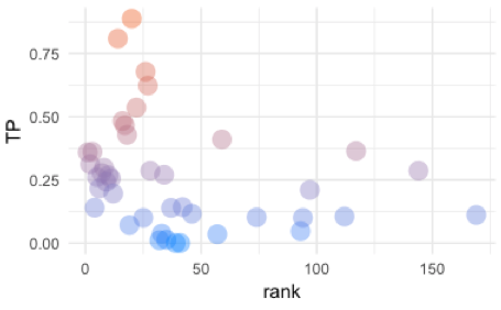
But when we plot, the non-linear correlation appears:

## Plotting relationship
ggplot(d_tp_rank, aes(rank, TP, color = TP)) +
  geom_point(shape = 16, size = 5, show.legend = FALSE, alpha = .4) +
  theme_minimal() +
  scale_color_gradient(low = "#0091ff", high = "#f0650e")

Biased model towards class with high rank

For those who are familiar with information theory, the last plot is a standard case of a functional relationship with some noise, (Ref. 1). Without looking at the reference, can you guess why? Is anything on the plot that give you a hint? Think about it 🤔

We can measure the information using the metric information gain ratio (gr variable), returned by the var_rank_info function (funModeling package):

var_rank_info(d_tp_rank, target = 'TP')

##    var    en    mi      ig        gr
## 1 rank 5.392 5.249 5.24946 0.9735073

Information gain ratio ranges from 0 to 1. A value closer to 1 indicates "more correlation" (or in information theory terms: the variable carries more information with the target).

Note: Don't confuse information gain ratio with information gain (wiki).

Going back to the example, we look at gr=0.97 it can be concluded that there is a relationship between sample size and accuracy.

And we know that deep learning needs lots of data.

How do we measure performance?

In the deep learning we get the model parameters by minimizng the loss value. Then the accuracy is calculated based on the recently trained model (Ref. 2).

It would be nice to check with another metric rather than the accuracy, just like Kappa, although it is not available on Keras by now, it is on caret.

Improving performance in high-unbalanced data

So the model will see a more balanced picture of what it needs to be learned.

For instance, if we are predicting 3-classes whose share are: A=2%, B=5%, and C=97%; we can take 100% of A, 100% of B, and a random sample of C.

Final distrubution could be: A=15%, B=35% and C=50%.

Results after balancing the classes

Next plot will show what happen when, for the same data, we balance the classes:

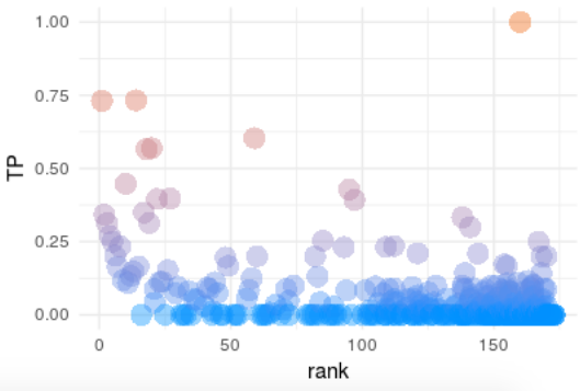
There are much more points, now the different classes that the model predicts are around 400. Which is a good signal because it shows that the model is trying to learn more unbalanced classes.

The other point is now the information gain ratio is 0.51. So we break down by almost 50% the dependency of sample size with the accuracy.

Altough it is not shown on this post, the overall accuracy has also been decreased, but now it it less biassed due to the classes with high rank.

Comparing the before and after:

Conclusions

What if last steps were not successful?

Even after choosing Kappa, or balancing the classes, we can find unsatisfactory results. However, the other explanation is "we don't have enough data to predict". But that should be the last option for a data scientist.
The method balancing method mentioned in this post was to assign weights to each class, this is supported semi-automatically in Keras through the class_weight parameter, but that is a topic for another post 😉.

The impact of representativeness:

It is shown in many topic across data projects, from power analysis in statistical test, in A/B testing analysis, when having more data (or a bigger effect size) makes the experiment to converge quicker.

Other cases in predictive modeling are the decision trees rules, when we analyze the support metric, or when we need to reduce the cardinality in a categorical variable to minimize the chance of overfitting (Ref. 3).