15 January 2019 / R

Feature Selection using Genetic Algorithms in R

This is a post about feature selection using genetic algorithms in R, in which we will do a quick review about:

What are genetic algorithms?
GA in ML?
What does a solution look like?
GA process and its operators
The fitness function
Genetics Algorithms in R!
Try it yourself
Relating concepts

Animation source: "Flexible Muscle-Based Locomotion for Bipedal Creatures" - Thomas Geijtenbeek

The intuition behind

Imagine a black box which can help us to decide over an unlimited number of possibilities, with a criterion such that we can find an acceptable solution (both in time and quality) to a problem that we formulate.

What are genetic algorithms?

Genetic Algortithms (GA) are a mathematical model inspired by the famous Charles Darwin's idea of natural selection.

The natural selection preserves only the fittest individuals, over the different generations.

Imagine a population of 100 rabbits in 1900, if we look the population today, we are going to others rabbits more fast and skillful to find food than their ancestors.

GA in ML

In machine learning, one of the uses of genetic algorithms is to pick up the right number of variables in order to create a predictive model.

To pick up the right subset of variables is a problem of combinatory and optimization.

The advantage of this technique over others is, it allows the best solution to emerge from the best of prior solutions. An evolutionary algorithm which improves the selection over time.

The idea of GA is to combine the different solutions generation after generation to extract the best genes (variables) from each one. That way it creates new and more fitted individuals.

We can find other uses of GA such as hyper-tunning parameter, find the maximum (or min) of a function or the search for a correct neural network arquitecture (Neuroevolution), or among others...

GA in feature selection

Every possible solution of the GA, which are the selected variables (a single 🐇), are considered as a whole, it will not rank variables individually against the target.

And this is important because we already know that variables work in group.

What does a solution look like?

Keeping it simple for the example, imagine we have a total of 6 variables,

One solution can be picking up 3 variables, let's say: var2, var4 and var5.

Another solution can be: var1 and var5.

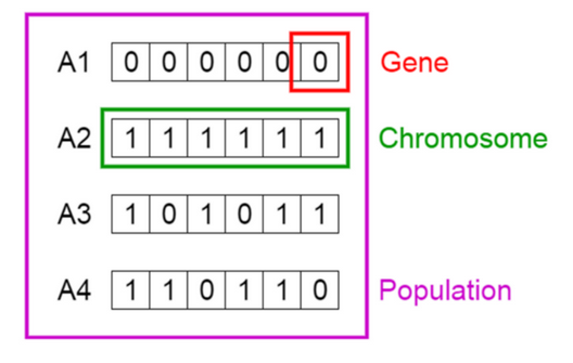
These solutions are the so-called individuals or chromosomes in a population. They are possible solutions to our problem.

Credit image: Vijini Mallawaarachchi

From the image, the solution 3 can be expressed as a one-hot vector: c(1,0,1,0,1,1). Each 1 indicates the solution containg that variable. In this case: var1, var3, var5, var6.

While the solution 4 is: c(1,1,0,1,1,0).

Each position in the vector is a gene.

GA process and its operators

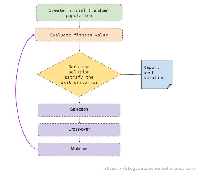
The underlying idea of a GA is to generate some random possible solutions (called population), which represent different variables, to then combine the best solutions in an iterative process.

This combination follows the basic GA operations, which are: selection, mutation and cross-over.

Selection: Pick up the most fitted individuals in a generation (i.e.: the solutions providing the highest ROC).
Cross-over: Create 2 new individuals, based on the genes of two solutions. These children will appear to the next generation.
Mutation: Change a gene randomly in the individual (i.e.: flip a 0 to 1)

The idea is for each generation, we will find better individuals, like a fast rabbit.

I recommend the post of Vijini Mallawaarachchi about how a genetic algorithm works.

These basic operations allow the algorithm to change the possible solutions by combining them in a way that maximizes the objective.

The fitness function

This objective maximization is, for example, to keep with the solution that maximizes the area under the ROC curve. This is defined in the fitness function.

The fitness function takes a possible solution (or chromosome, if you want to sound more sophisticated), and somehow evaluates the effectiveness of the selection.

Normally, the fitness function takes the one-hot vector c(1,1,0,0,0,0), creates, for example, a random forest model with var1 and var2, and returns the fitness value (ROC).

The fitness value in this code calculates is: ROC value / number of variables. By doing this the algorithm penalizes the solutions with a large number of variables. Similar to the idea of Akaike information criterion, or AIC.

Genetics Algorithms in R! 🐛

My intention is to provide you with a clean code so you can understand what's behind, while at the same time, try new approaches like modifying the fitness function. This is a crucial point.

To use on your own data set, make sure data_x (data frame) and data_y (factor) are compatible with the custom_fitness function.

The main library is GA, developed by Luca Scrucca. See here the vignette with examples.

📣 Important: The following code is incomplete. Clone the repository to run the example.

# data_x: input data frame
# data_y: target variable (factor)

# GA parameters
param_nBits=ncol(data_x)
col_names=colnames(data_x)

# Executing the GA 
ga_GA_1 = ga(fitness = function(vars) custom_fitness(vars = vars, 
                                                     data_x =  data_x, 
                                                     data_y = data_y, 
                                                     p_sampling = 0.7), # custom fitness function
             type = "binary", # optimization data type
             crossover=gabin_uCrossover,  # cross-over method
             elitism = 3, # best N indiv. to pass to next iteration
             pmutation = 0.03, # mutation rate prob
             popSize = 50, # the number of indivduals/solutions
             nBits = param_nBits, # total number of variables
             names=col_names, # variable name
             run=5, # max iter without improvement (stopping criteria)
             maxiter = 50, # total runs or generations
             monitor=plot, # plot the result at each iteration
             keepBest = TRUE, # keep the best solution at the end
             parallel = T, # allow parallel procesing
             seed=84211 # for reproducibility purposes
)

# Checking the results
summary(ga_GA_1)

── Genetic Algorithm ─────────────────── 

GA settings: 
Type                  =  binary 
Population size       =  50 
Number of generations =  50 
Elitism               =  3 
Crossover probability =  0.8 
Mutation probability  =  0.03 

GA results: 
Iterations             = 17 
Fitness function value = 0.2477393 
Solution = 
     radius_mean texture_mean perimeter_mean area_mean smoothness_mean compactness_mean
[1,]           0            1              0         0               0                1
     concavity_mean concave points_mean symmetry_mean fractal_dimension_mean  ... 
[1,]              0                   0             0                      0      
     symmetry_worst fractal_dimension_worst
[1,]              0                       0

# Following line will return the variable names of the final and best solution
best_vars_ga=col_names[ga_GA_1@solution[1,]==1]

# Checking the variables of the best solution...
best_vars_ga

[1] "texture_mean"     "compactness_mean" "area_worst"       "concavity_worst"

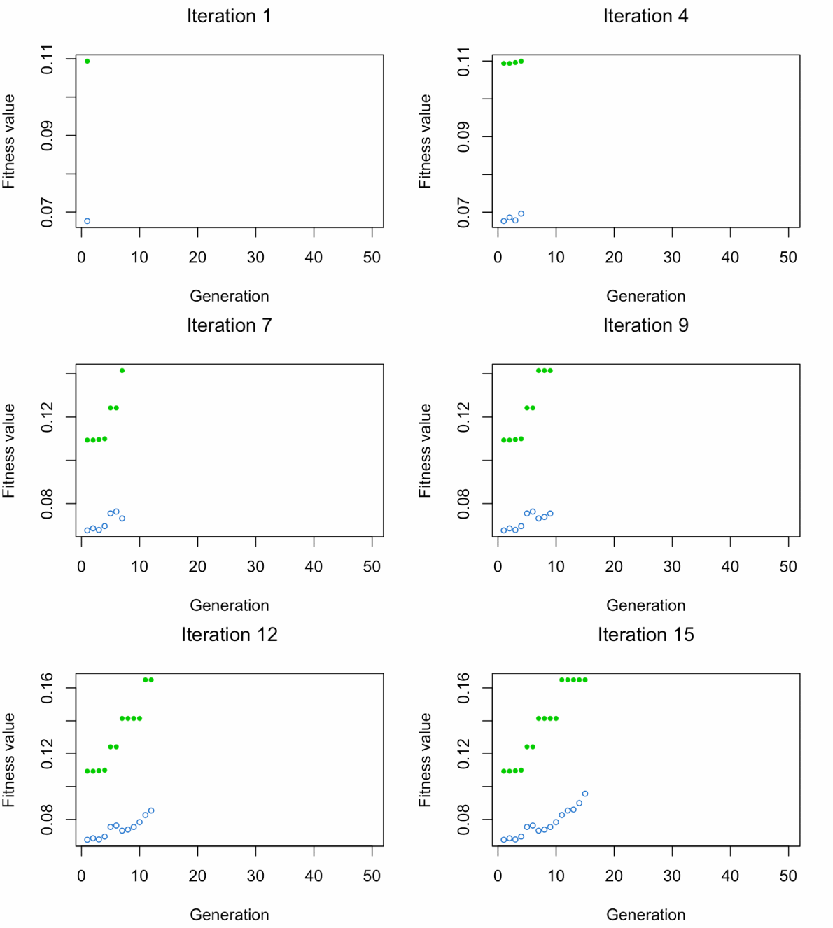
Blue dot: Population fitness average
Green dot: Best fitness value

Note: Don't expect the result that fast 😅

Now we calculate the accuracy based on the best selection!

get_accuracy_metric(data_tr_sample = data_x, target = data_y, best_vars_ga)

[1] 0.9508279

The accuracy is around 95,08%, while the ROC value is closed to 0,95 (ROC=fitness value * number of variables, check the fitness function).

Analyzing the results

I don't like to analyze the accuracy without the cutpoint (Scoring Data), but it's useful to compare with the results of this Kaggle post.

He got a similar accuracy result using recursive feature elimination, or RFE, based on 5 variables, while our solution stays with 4.

Try it yourself

Try a new fitness function, some solutions still provide a large number of variables, you can try squaring the number of variables.

Another thing to try is the algorithm to get the ROC value, or even to change the metric.

Some configurations last a lot of time. Balance classes before modeling and play with the p_sampling parameter. Sampling techniques can have a big impact on models. Check the Sample size and class balance on model performance post for more info.

How about changing the rate of mutation or elitism? Or trying other cross-over methods?

Increase the popSize to test more possible solutions at the same time (at a time cost).

Feel free to share any insights or ideas to improve the selection.

Clone the repository to run the example.

Relating concepts

There is a parallelism between GA and Deep Learning, the concept of iteration and improvement over time is similar.

I added the p_sampling parameter to speed up things. And it usually accomplishes its goal. Similar to the batch concept used in Deep Learning. Another parallel is between the GA parameter run and the early stopping criteria in the neural network training.

But the biggest similarity is both techniques come from observing the nature. In both cases, humans observed how neural networks and genetics work, and create a simplified mathematical model that imitate their behavior. Nature has millions of years of evolution, why not try to imitate it? 🌱

I tried to be brief about GA, but if you have any specific question on this vast topic, please leave it in the comments 🙋 🙋‍♂

And, if I didn't motivate you the enough to study GA, check this project which is based on Neuroevolution:

Thanks for reading 🚀

Find me on Twitter and Linkedin.
More blog posts.

Want to learn more? 📗 Data Science Live Book