Exploratory Data Analysis in R (introduction)
Hi there!
tl;dr: Exploratory data analysis (EDA) the very first step in a data project. We will create a code-template to achieve this with one function.
Introduction
EDA consists of univariate (1-variable) and bivariate (2-variables) analysis.
In this post we will review some functions that lead us to the analysis of the first case.
- Step 1 - First approach to data
- Step 2 - Analyzing categorical variables
- Step 3 - Analyzing numerical variables
- Step 4 - Analyzing numerical and categorical at the same time
Covering some key points in a basic EDA:
- Data types
- Outliers
- Missing values
- Distributions (numerically and graphically) for both, numerical and categorical variables.
Type of analysis results
They can be two: informative or operative.
Informative - For example plots, or any long variable summary. We cannot filter data from it, but give us a lot of information at once. Most used on the EDA stage.
Operative - The results can be used to take an action directly on the data workflow (for example, selecting any variables whose percentage of missing values are below 20%). Most used in the Data Preparation stage.
Setting-up
Uncoment in case you don't have any of these libraries:
# install.packages("tidyverse")
# install.packages("funModeling")
# install.packages("Hmisc")
A newer version of funModeling has been released on Ago-1, please update ;)
Now load the needed libraries...
library(funModeling)
library(tidyverse)
library(Hmisc)
tl;dr (code)
Run all the functions in this post in one-shot with the following function:
basic_eda <- function(data)
{
  glimpse(data)
  print(status(data))
  freq(data)
  print(profiling_num(data))
  plot_num(data)
  describe(data)
}
Replace data with your data, and that's it!:
basic_eda(my_amazing_data)
Creating the data for this example
Using the heart_disease data (from funModeling package). We will take only 4 variables for legibility.
data=heart_disease %>% select(age, max_heart_rate, thal, has_heart_disease)
Step 1 - First approach to data
Number of observations (rows) and variables, and a head of the first cases.
glimpse(data)
## Observations: 303
## Variables: 4
## $ age               <int> 63, 67, 67, 37, 41, 56, 62, 57, 63, 53, 57, ...
## $ max_heart_rate    <int> 150, 108, 129, 187, 172, 178, 160, 163, 147,...
## $ thal              <fct> 6, 3, 7, 3, 3, 3, 3, 3, 7, 7, 6, 3, 6, 7, 7,...
## $ has_heart_disease <fct> no, yes, yes, no, no, no, yes, no, yes, yes,...
Getting the metrics about data types, zeros, infinite numbers, and missing values:
status(data)
##            variable q_zeros p_zeros q_na p_na   q_inf p_inf    type unique
## 1               age       0       0    0 0.0000     0     0 integer     41
## 2    max_heart_rate       0       0    0 0.0000     0     0 integer     91
## 3              thal       0       0    2 0.0066     0     0  factor      3
## 4 has_heart_disease       0       0    0 0.0000     0     0  factor      2
status returns a table, so it is easy to keep with variables that match certain conditions like:
+ Having at least 80% of non-NA values (p_na < 0.2)
+ Having less than 50 unique values (unique <= 50)
💡 TIPS:
- Are all the variables in the correct data type?
- Variables with lots of zeros or
NAs? - Any high cardinality variable?
[🔎 Read more here.]
Step 2 - Analyzing categorical variables
freq function runs for all factor or character variables automatically:
freq(data)
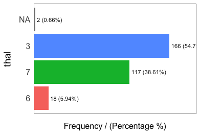
##   thal frequency percentage cumulative_perc
## 1    3       166      54.79              55
## 2    7       117      38.61              93
## 3    6        18       5.94              99
## 4 <NA>         2       0.66             100
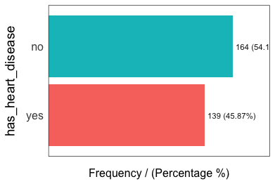
##   has_heart_disease frequency percentage cumulative_perc
## 1                no       164         54              54
## 2               yes       139         46             100
## [1] "Variables processed: thal, has_heart_disease"
💡 TIPS:
- If
freqreceives one variable -freq(data$variable)- it retruns a table. Useful to treat high cardinality variables (like zip code). - Export the plots to jpeg into current directory:
freq(data, path_out = ".") - Does all the categories make sense?
- Lots of missing values?
- Always check absolute and relative values
[🔎 Read more here.]
Step 3 - Analyzing numerical variables
We will see: plot_num and profiling_num. Both run automatically for all numerical/integer variables:
Graphically
plot_num(data)
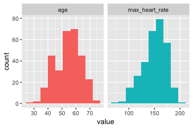
Export the plot to jpeg: plot_num(data, path_out = ".")
💡 TIPS:
- Try to identify high-unbalanced variables
- Visually check any variable with outliers
[🔎 Read more here.]
Quantitatively
profiling_num runs for all numerical/integer variables automatically:
data_prof=profiling_num(data)
##         variable mean std_dev variation_coef p_01 p_05 p_25 p_50 p_75 p_95
## 1            age   54       9           0.17   35   40   48   56   61   68
## 2 max_heart_rate  150      23           0.15   95  108  134  153  166  182
##   p_99 skewness kurtosis iqr        range_98     range_80
## 1   71    -0.21      2.5  13        [35, 71]     [42, 66]
## 2  192    -0.53      2.9  32 [95.02, 191.96] [116, 176.6]
💡 TIPS:
- Try to describe each variable based on its distribution (also useful for reporting)
- Pay attention to variables with high standard deviation.
- Select the metrics that you are most familiar with:
data_prof %>% select(variable, variation_coef, range_98): A high value invariation_coefmay indictate outliers.range_98indicates where most of the values are.
[🔎 Read more here.]
Step 4 - Analyzing numerical and categorical at the same time
describe from Hmisc package.
library(Hmisc)
describe(data)
## data
##
##  4  Variables      303  Observations
## ---------------------------------------------------------------------------
## age
##        n  missing distinct     Info     Mean      Gmd      .05      .10
##      303        0       41    0.999    54.44     10.3       40       42
##      .25      .50      .75      .90      .95
##       48       56       61       66       68
##
## lowest : 29 34 35 37 38, highest: 70 71 74 76 77
## ---------------------------------------------------------------------------
## max_heart_rate
##        n  missing distinct     Info     Mean      Gmd      .05      .10
##      303        0       91        1    149.6    25.73    108.1    116.0
##      .25      .50      .75      .90      .95
##    133.5    153.0    166.0    176.6    181.9
##
## lowest :  71  88  90  95  96, highest: 190 192 194 195 202
## ---------------------------------------------------------------------------
## thal
##        n  missing distinct
##      301        2        3
##
## Value         3    6    7
## Frequency   166   18  117
## Proportion 0.55 0.06 0.39
## ---------------------------------------------------------------------------
## has_heart_disease
##        n  missing distinct
##      303        0        2
##
## Value        no  yes
## Frequency   164  139
## Proportion 0.54 0.46
## ---------------------------------------------------------------------------
Really useful to have a quick picture for all the variables. But is not as operative as freq and profiling_num when we want to use its results to change our data workflow.
💡 TIPS:
- Check min and max values (outliers)
- Check Distributions (same as before)
[🔎 Read more here.]
That's all by now! :)
PC.
Other posts you might like: